Summarizing Embeddings for Administrative Regions • GeoTessera

Introduction

When working with large geographic regions, you often need summary statistics rather than full pixel-level embeddings. The summarize_region() method provides a pipeline that:

Downloads embeddings to a temporary location
Optionally masks pixels to match irregular region boundaries
Computes user-specified summary statistics
Automatically cleans up downloaded data

This vignette demonstrates how to use this functionality with administrative boundaries from a shapefile.

Setup

library(GeoTessera)
library(sf)
library(ggplot2)

Demonstration with Simulated Data

Before working with real data, let’s demonstrate the summarization workflow with simulated embeddings and regions.

Creating Example Regions

# Create 4 example polygon regions (simulating LGAs)
region1 <- st_polygon(list(matrix(c(
  0, 0, 1, 1, 0,
  0, 1, 1, 0, 0
), ncol = 2))) |> st_sfc(crs = 4326)

region2 <- st_polygon(list(matrix(c(
  1, 1, 2, 2, 1,
  0, 1, 1, 0, 0
), ncol = 2))) |> st_sfc(crs = 4326)

region3 <- st_polygon(list(matrix(c(
  0, 0, 1, 1, 0,
  1, 2, 2, 1, 1
), ncol = 2))) |> st_sfc(crs = 4326)

region4 <- st_polygon(list(matrix(c(
  1, 1, 2, 2, 1,
  1, 2, 2, 1, 1
), ncol = 2))) |> st_sfc(crs = 4326)

# Combine into sf object
regions <- st_sf(
  name = c("Region A", "Region B", "Region C", "Region D"),
  land_type = c("urban", "agricultural", "forest", "mixed"),
  geometry = c(region1, region2, region3, region4)
)

# Plot the regions
ggplot(regions) +
  geom_sf(aes(fill = land_type), alpha = 0.7) +
  geom_sf_text(aes(label = name), size = 4) +
  scale_fill_manual(values = c("urban" = "#E41A1C",
                                "agricultural" = "#FFD92F",
                                "forest" = "#4DAF4A",
                                "mixed" = "#984EA3")) +
  labs(title = "Example Administrative Regions",
       subtitle = "Simulating 4 LGAs with different land cover types") +
  theme_minimal()
#> Warning in st_point_on_surface.sfc(sf::st_zm(x)): st_point_on_surface may not
#> give correct results for longitude/latitude data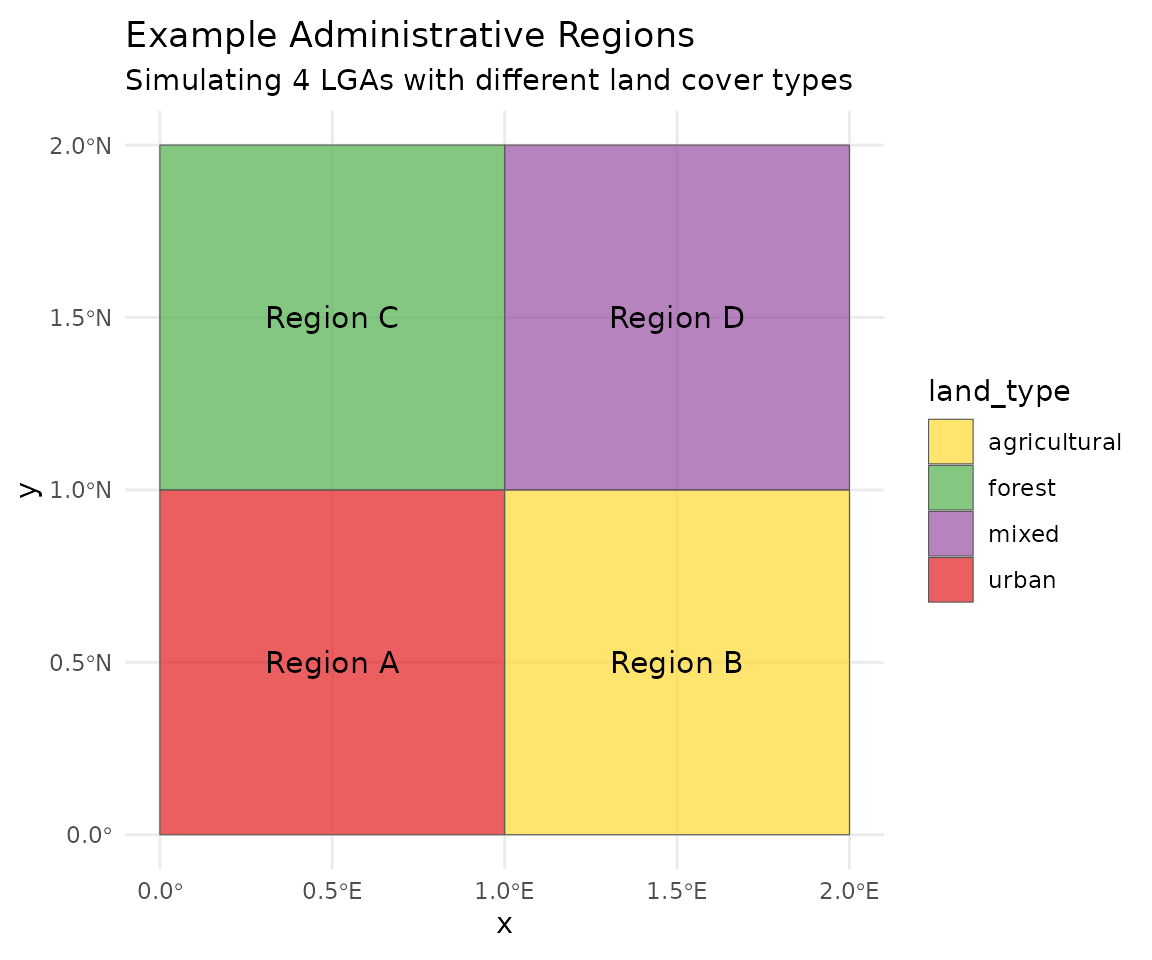

Simulating Region Embeddings

set.seed(42)

# Simulate mean embeddings for each region type
# Different land types have distinct embedding signatures
simulate_embedding <- function(land_type) {
  base <- switch(land_type,
    "urban" = rnorm(128, mean = 0.5, sd = 0.1),
    "agricultural" = rnorm(128, mean = 0.0, sd = 0.15),
    "forest" = rnorm(128, mean = -0.4, sd = 0.12),
    "mixed" = rnorm(128, mean = 0.1, sd = 0.2)
  )
  base
}

# Generate embeddings for each region
region_embeddings <- lapply(regions$land_type, simulate_embedding)
names(region_embeddings) <- regions$name

# Create embedding matrix
emb_matrix <- do.call(rbind, region_embeddings)
rownames(emb_matrix) <- regions$name

cat("Embedding matrix dimensions:", dim(emb_matrix), "\n")
#> Embedding matrix dimensions: 4 128
cat("Rows:", rownames(emb_matrix), "\n")
#> Rows: Region A Region B Region C Region D

Region Similarity Heatmap

# Calculate cosine similarity between regions
cosine_sim <- function(a, b) {
  sum(a * b) / (sqrt(sum(a^2)) * sqrt(sum(b^2)))
}

n_regions <- nrow(emb_matrix)
sim_matrix <- matrix(0, n_regions, n_regions)
for (i in 1:n_regions) {
  for (j in 1:n_regions) {
    sim_matrix[i, j] <- cosine_sim(emb_matrix[i, ], emb_matrix[j, ])
  }
}
rownames(sim_matrix) <- colnames(sim_matrix) <- regions$name

# Convert to data frame for plotting
sim_df <- as.data.frame(as.table(sim_matrix))
names(sim_df) <- c("Region1", "Region2", "Similarity")

ggplot(sim_df, aes(x = Region1, y = Region2, fill = Similarity)) +
  geom_tile() +
  geom_text(aes(label = round(Similarity, 2)), color = "white", size = 4) +
  scale_fill_gradient2(low = "blue", mid = "white", high = "red", midpoint = 0.5) +
  labs(title = "Region Similarity Matrix",
       subtitle = "Cosine similarity based on mean embeddings") +
  theme_minimal() +
  theme(axis.text.x = element_text(angle = 45, hjust = 1))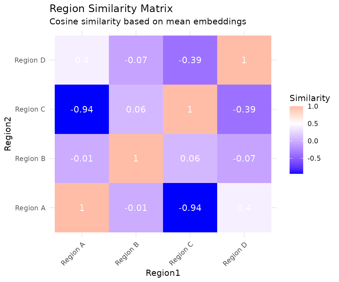

Embedding Profile Comparison

# Compare first 20 dimensions across regions
profile_df <- data.frame(
  Dimension = rep(1:20, 4),
  Value = c(emb_matrix[1, 1:20], emb_matrix[2, 1:20],
            emb_matrix[3, 1:20], emb_matrix[4, 1:20]),
  Region = rep(regions$name, each = 20)
)

ggplot(profile_df, aes(x = Dimension, y = Value, color = Region)) +
  geom_line(linewidth = 1) +
  geom_point(size = 2) +
  scale_color_brewer(palette = "Set1") +
  labs(title = "Embedding Profiles by Region",
       subtitle = "First 20 of 128 dimensions shown",
       x = "Embedding Dimension", y = "Value") +
  theme_minimal() +
  theme(legend.position = "bottom")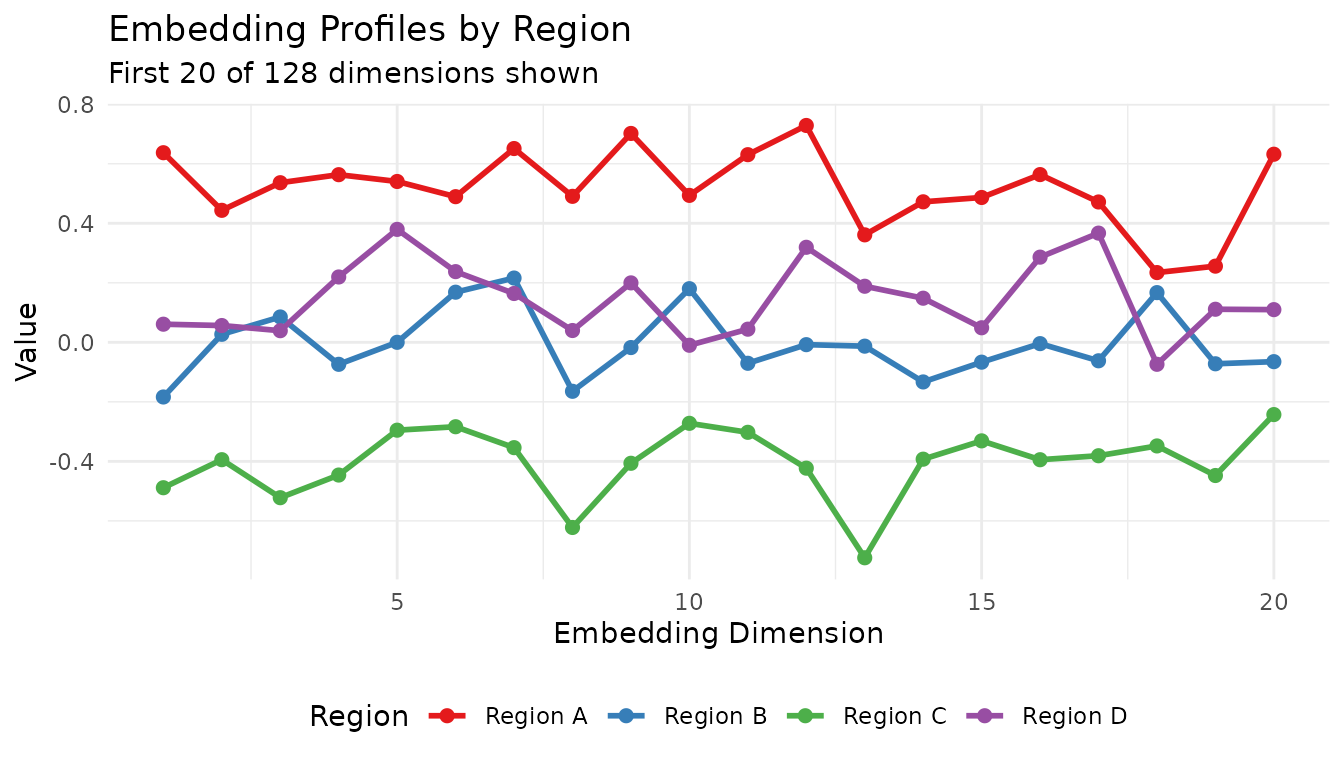

Hierarchical Clustering of Regions

# Cluster regions by embedding similarity
dist_matrix <- dist(emb_matrix)
hc <- hclust(dist_matrix, method = "ward.D2")

# Simple dendrogram plot
plot(hc, main = "Hierarchical Clustering of Regions",
     sub = "Based on 128-dimensional embeddings",
     xlab = "", ylab = "Distance")

Map with Cluster Assignment

# Cut tree into 2 clusters
regions$cluster <- factor(cutree(hc, k = 2))

ggplot(regions) +
  geom_sf(aes(fill = cluster), alpha = 0.7) +
  geom_sf_text(aes(label = paste0(name, "\n(", land_type, ")")), size = 3) +
  scale_fill_brewer(palette = "Set2") +
  labs(title = "Regions Clustered by Embedding Similarity",
       subtitle = "Regions with similar land cover cluster together") +
  theme_minimal()
#> Warning in st_point_on_surface.sfc(sf::st_zm(x)): st_point_on_surface may not
#> give correct results for longitude/latitude data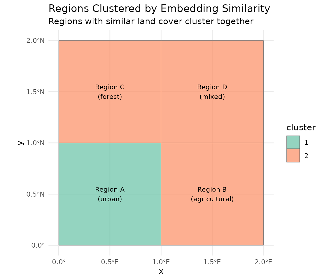

Loading Administrative Boundaries

We’ll use Nigeria’s Local Government Areas (LGAs) as an example. This shapefile contains 774 administrative units at the admin2 level.

# Load the shapefile
nigeria_lgas <- st_read("shapefiles/nigeria_admin2_shapefile.shp", quiet = TRUE)

# Examine the structure
print(nigeria_lgas[1:5, c("adminCode", "adminName")])

Simple feature collection with 5 features and 2 fields
  adminCode      adminName                       geometry
1  NG001001      Aba North MULTIPOLYGON (((7.401109 5....
2  NG001002      Aba South MULTIPOLYGON (((7.387495 5....
3  NG015001          Abaji MULTIPOLYGON (((7.045872 9....
4  NG003001           Abak MULTIPOLYGON (((7.811244 5....
5  NG011001      Abakaliki MULTIPOLYGON (((8.4109 6.28...

Summarizing a Single LGA

Let’s compute embedding summaries for Aba North, a small LGA in southeastern Nigeria.

# Select Aba North LGA
aba_north <- nigeria_lgas[nigeria_lgas$adminName == "Aba North", ]

# View the region
plot(st_geometry(aba_north), main = "Aba North LGA", col = "lightblue")

Basic Summary

The summarize_region() method accepts an sf object directly. It will:

Use the bounding box to determine which tiles to download
Mask pixels outside the polygon boundary
Compute summary statistics

# Create GeoTessera client
gt <- geotessera()

# Compute summaries for Aba North
result <- gt$summarize_region(
  region = aba_north,
  year = 2024
)

# View the structure
names(result)
# [1] "summaries" "metadata"

# View metadata
result$metadata
# $region_bbox
# [1]  7.331234  5.081948  7.402708  5.134542
#
# $year
# [1] 2024
#
# $n_tiles
# [1] 4
#
# $is_masked
# [1] TRUE

Default Summary Statistics

By default, summarize_region() computes three summaries:

# Mean embedding (128-dimensional vector)
mean_embedding <- result$summaries$mean
length(mean_embedding)
# [1] 128

# First 10 dimensions
head(mean_embedding, 10)

# Centroid embedding (sampled at geographic center)
centroid_embedding <- result$summaries$centroid
length(centroid_embedding)
# [1] 128

# Coverage statistics
result$summaries$coverage
# n_tiles    n_valid_pixels n_total_pixels coverage_percent
#       4           xxxxx          xxxxx            xx.xx

Custom Summary Functions

You can specify which summary functions to use, including custom ones.

Built-in Summary Functions

GeoTessera provides several built-in summary functions:

Function	Description
`summary_mean`	Mean across all pixels
`summary_median`	Median across all pixels
`summary_sd`	Standard deviation per dimension
`summary_centroid`	Sample at geographic centroid
`summary_pixel_count`	Count of valid/total pixels
`summary_coverage`	Coverage statistics
`summary_quantile(probs)`	Factory for quantile summaries
`summary_random_sample(n, seed)`	Factory for random sampling

# Use specific summary functions
result <- gt$summarize_region(
  region = aba_north,
  year = 2024,
  summary_fns = list(
    mean = summary_mean,
    median = summary_median,
    sd = summary_sd,
    coverage = summary_coverage
  )
)

# Standard deviation tells us about embedding variability
sd_embedding <- result$summaries$sd
summary(sd_embedding)

Quantile Summaries

Use summary_quantile() to create a function that computes specific quantiles:

# Create a function for 10th and 90th percentiles
result <- gt$summarize_region(
  region = aba_north,
  year = 2024,
  summary_fns = list(
    q10_90 = summary_quantile(c(0.10, 0.90))
  )
)

# Returns 256 values (128 dimensions × 2 quantiles)
length(result$summaries$q10_90)

Random Sampling

Use summary_random_sample() to extract random pixel embeddings:

# Sample 50 random pixels (reproducible with seed)
result <- gt$summarize_region(
  region = aba_north,
  year = 2024,
  summary_fns = list(
    samples = summary_random_sample(n = 50, seed = 42)
  )
)

# Returns a matrix: 50 samples × 128 dimensions
dim(result$summaries$samples)
# [1]  50 128

Custom Summary Functions

Create your own summary function. It should accept:

embeddings: List of 3D arrays (height × width × 128)
region: The input region (sf object or bbox)
tiles_df: Tile metadata data frame

# Custom function: compute the embedding at the pixel with maximum brightness
# (using sum across channels as a proxy for "brightness")
summary_max_brightness <- function(embeddings, region = NULL, tiles_df = NULL) {
  max_sum <- -Inf
  max_embedding <- NULL

  for (emb in embeddings) {
    # Sum across channels for each pixel
    pixel_sums <- apply(emb, c(1, 2), sum, na.rm = TRUE)

    # Find max
    max_idx <- which.max(pixel_sums)
    if (pixel_sums[max_idx] > max_sum) {
      max_sum <- pixel_sums[max_idx]
      # Convert linear index to array indices
      idx <- arrayInd(max_idx, dim(pixel_sums))
      max_embedding <- emb[idx[1], idx[2], ]
    }
  }

  names(max_embedding) <- paste0("dim_", seq_along(max_embedding))
  max_embedding
}

# Use the custom function
result <- gt$summarize_region(
  region = aba_north,
  year = 2024,
  summary_fns = list(
    mean = summary_mean,
    max_brightness = summary_max_brightness
  )
)

Processing Multiple Regions

When processing multiple regions, adjacent areas often share tiles. GeoTessera provides an optimized summarize_regions_streaming() function that:

Builds a region-to-tile mapping - identifies which tiles each region needs
Detects shared tiles - finds tiles used by multiple regions
Optimizes download order - processes most-shared tiles first
Downloads each tile only once - even if multiple regions need it
Uses streaming statistics - constant memory regardless of region size

Efficient Multi-Region Processing

# Select adjacent LGAs that share tiles
selected_lgas <- c("Aba North", "Aba South", "Osisioma Ngwa", "Ugwunagbo")
lgas_subset <- nigeria_lgas[nigeria_lgas$adminName %in% selected_lgas, ]

# Process all regions efficiently
result <- summarize_regions_streaming(

  gt = gt,
  regions = lgas_subset,
  year = 2024,
  region_ids = lgas_subset$adminName,
  sample_rate = 0.1,      # Sample 10% of pixels for speed
  mask_to_region = TRUE   # Only include pixels inside each polygon
)

# View optimization statistics
result$metadata
# $n_regions
# [1] 4
#
# $n_unique_tiles
# [1] 11
#
# $tiles_downloaded
# [1] 11
#
# (4 tiles were shared between regions - downloaded only once!)

The function returns:

summaries: Named list of mean embeddings (128-dim vector per region)
pixel_counts: Number of pixels processed per region
metadata: Processing statistics

# Access results for a specific region
aba_north_embedding <- result$summaries[["Aba North"]]
length(aba_north_embedding)
# [1] 128

# View pixel counts
result$pixel_counts
#     Aba North     Aba South Osisioma Ngwa     Ugwunagbo
#         18800         43538        175735        126769

# Combine into a matrix for analysis
embedding_matrix <- do.call(rbind, result$summaries)
dim(embedding_matrix)
# [1]   4 128

Comparison: Sequential vs Optimized

For adjacent regions, the optimized approach is significantly faster:

Sequential processing (4 LGAs separately):
  - Each LGA downloads its own tiles
  - Shared tiles downloaded multiple times
  - Total: ~20+ tile downloads

Optimized streaming (summarize_regions_streaming):
  - Builds tile sharing graph
  - Downloads each unique tile once
  - Total: 11 tile downloads (4 shared)

Large-Scale Processing

For processing many regions (e.g., all LGAs in a country), use sampling to reduce processing time:

# Process all LGAs in a state
abia_lgas <- nigeria_lgas[grepl("^NG001", nigeria_lgas$adminCode), ]

result <- summarize_regions_streaming(
  gt = gt,
  regions = abia_lgas,
  year = 2024,
  region_ids = abia_lgas$adminName,
  sample_rate = 0.05,     # 5% sampling for very large jobs
  mask_to_region = TRUE
)

Creating a Summary Data Frame

Combine embeddings with administrative metadata:

# Create data frame with LGA info and embeddings
embedding_matrix <- do.call(rbind, result$summaries)
lga_embeddings <- data.frame(
  adminName = names(result$summaries),
  embedding_matrix
)

# Add area information
lga_embeddings$area_km2 <- as.numeric(st_area(lgas_subset)) / 1e6

# Now you can use this for clustering, classification, etc.
head(lga_embeddings[, 1:5])

Controlling Masking Behavior

By default, pixels outside the region boundary are masked (set to NA). You can disable this to include all pixels within the bounding box:

# Without masking - uses rectangular bounding box
result_unmasked <- gt$summarize_region(
  region = aba_north,
  year = 2024,
  mask_to_region = FALSE
)

# With masking (default) - only pixels inside the polygon
result_masked <- gt$summarize_region(
  region = aba_north,
  year = 2024,
  mask_to_region = TRUE
)

# Compare coverage
result_unmasked$summaries$coverage["n_valid_pixels"]
result_masked$summaries$coverage["n_valid_pixels"]
# Masked version will have fewer valid pixels

Using Bounding Boxes

You can also use simple bounding boxes instead of sf objects:

# Define a bounding box (xmin, ymin, xmax, ymax)
bbox <- c(7.33, 5.08, 7.40, 5.14)

result <- gt$summarize_region(
  region = bbox,
  year = 2024
)

# Note: masking is not applied for bounding boxes
result$metadata$is_masked
# [1] FALSE

Performance Considerations

Temporary File Management

Downloaded tiles are stored in a temporary directory and automatically cleaned up when summarize_region() completes. If you need to keep the tiles:

result <- gt$summarize_region(
  region = aba_north,
  year = 2024,
  keep_tiles = TRUE
)

# Access the downloaded Tile objects
tiles <- result$tiles
length(tiles)

# Load embedding from first tile
emb <- tiles[[1]]$load_embedding()
dim(emb)

Large Regions (Memory-Efficient Streaming)

For very large regions (many tiles), the standard summarize_region() may run out of memory because it loads all embeddings before computing statistics.

Use summarize_region_streaming() for memory-efficient processing of large single regions:

# Abaji LGA requires 36 tiles - too large for standard approach
abaji <- nigeria_lgas[nigeria_lgas$adminName == "Abaji", ]

# Use streaming approach - processes one tile at a time
result <- gt$summarize_region_streaming(
 region = abaji,
  year = 2024,
  sample_rate = 0.1,       # Sample 10% of pixels
  mask_to_region = FALSE   # Skip masking for speed
)

# Results
result$mean          # 128-dimensional mean embedding
result$n_pixels      # Number of pixels processed
result$metadata$processing_time_secs

The streaming approach:

Constant memory: Processes one tile at a time using Welford’s online algorithm
Sampling support: Reduce processing time with sample_rate < 1.0
No memory issues: Successfully handles regions with 30+ tiles

Alternative: Point Sampling Within Polygon

Another memory-efficient approach is to sample random points within the polygon and fetch their embeddings:

# Sample 1000 random points inside the polygon
set.seed(42)
sample_points <- st_sample(abaji, size = 1000)
coords <- st_coordinates(sample_points)
points_df <- data.frame(lon = coords[, 1], lat = coords[, 2])

# Fetch embeddings at those points
embeddings_df <- gt$sample_embeddings_at_points(points_df, year = 2024)

# Compute mean (excluding lon/lat columns)
mean_embedding <- colMeans(embeddings_df[, -(1:2)], na.rm = TRUE)

Example: Clustering LGAs by Land Cover Similarity

Here’s a complete example that clusters Nigerian LGAs based on embedding similarity, using the optimized multi-region streaming approach:

library(GeoTessera)
library(sf)

# Load shapefile
nigeria_lgas <- st_read("shapefiles/nigeria_admin2_shapefile.shp", quiet = TRUE)

# Calculate areas and select small LGAs for demo
nigeria_lgas$area_km2 <- as.numeric(st_area(nigeria_lgas)) / 1e6
small_lgas <- nigeria_lgas[nigeria_lgas$area_km2 < 100, ]
small_lgas <- small_lgas[1:20, ]  # Take first 20 for demo

# Initialize client
gt <- geotessera()

# Compute mean embeddings for all LGAs efficiently
# This optimizes tile downloads when regions share tiles
result <- summarize_regions_streaming(
  gt = gt,
  regions = small_lgas,
  year = 2024,
  region_ids = small_lgas$adminName,
  sample_rate = 0.1,
  mask_to_region = TRUE
)

# Create embedding matrix from results
emb_matrix <- do.call(rbind, result$summaries)

# Hierarchical clustering
dist_matrix <- dist(emb_matrix)
hc <- hclust(dist_matrix, method = "ward.D2")

# Plot dendrogram
plot(hc, main = "LGA Clustering by Embedding Similarity",
     xlab = "", sub = "")

# Cut into clusters
clusters <- cutree(hc, k = 4)

# Add cluster assignments back to spatial data
small_lgas$cluster <- clusters[small_lgas$adminName]

# Plot clusters on map
plot(small_lgas["cluster"], main = "LGA Clusters")

Summary

The summarize_region() method provides a convenient pipeline for:

Downloading embeddings for arbitrary regions
Masking to irregular boundaries from shapefiles
Computing flexible summary statistics
Cleaning up temporary files automatically

This enables analysis workflows where you need region-level embeddings rather than full pixel-level data, such as:

Administrative unit characterization
Regional clustering and classification
Time series analysis at the regional level
Feature extraction for machine learning models